
Programming Collective Intelligence chapter 5 notes
Published: 2014-04-19
Tagged: python readings guide
This chapter of Programming Collective Intelligence (from here on referred to as The Book) delves into the world of optimization and how to use it to find efficient solutions.
The examples featured in this chapter explain the meaning of efficient solutions. First, we tackle the problem of finding the best flights for a group of people who want to meet on the same day. Then we solve the problem of a group of students who want dorms - how do you make everyone happy if students have different preferences. Finally, we see how we can graph connections between social media users with the minimum amount of criss-crossed lines.
All of these problems have one thing in common: cost. The cost shows how good or bad a combination of items is. Using the example outlined above, the cost reflects the waiting time and ticket costs for the people who want to meet; how good students fit their dorms - ie. if students are assigned their least preferred dorms, the cost will be high; the higher the number of criss-crossed lines in our graph, the higher the cost.
Our aim in all of these cases is to minimize these costs. The Book introduces four ways that accomplish this. The code is really good at illustrating how exactly these methods work. On a side note, this chapter is similar to the first two weeks of Andrew Ng's coursera Machine Learning course, except that The Book focuses more on showing the code and intuition whereas Andrew Ng focuses on the math behind it. I think that covering both is the way to go, as both approaches highlighted different aspects of the same problem for me. The course was fairly strict in how it defined the cost function, whereas The Book put emphasis on intuitively defining it.
Optimization
To start, I'll go over the four optimization techniques that The Book introduces in optimization.py. Having a set of inputs, we can calculate all of their possible values sequentially and obtain the lowest cost. However, this isn't a method suitable for real-world scenarios where our inputs might number in the hundreds, thousands, or millions. It would take a huge amount of time to test each possible combination to arrive at the most cost efficient one. Hence the need for techniques that achieve our goal in a limited number of calculations. By the way - by formatting the input data the right way, we can use these functions for each example problem in this chapter.
The first technique is the function called random_optimize. As the name implies, it combines the inputs in random sets and tests the costs of those sets. It does this ten thousand times and returns the set that gave us the lowest cost. It gives us a better chance of finding the lowest cost than the sequential approach, but because of the randomness, we can't rely on it to give us the lowest cost each time we try.
The second technique is called hill_climb. The technique evaluates an initial random input set and then iteratively introduces small changes to this set. If a change has lowered the cost, it is "saved" and then another change is introduces. If a change has increased the cost, then the change is rolled back. This process repeats itself until no changes occur. In other words, this technique will find a local optimum, or the place where the cost is lowest.
The third technique, annealing_optimize, tries to figure out the global optimum. This is a huge improvement over the previous technique, as the global optimum is the lowest possible cost. It's a bit more complicated than hill climb, but it's well worth it.
Simulated annealing uses the same mechanism of starting out at a random solution and then trying out small changes. These changes give either a higher or lower cost relative to the initial solution. Unlike hill climb, this algorithm introduces the notion of 'temperature', which is used to calculate the probability of accepting a higher cost. The algorithm starts with a high temperature and slowly decreases it. As the temperature decreases, the probability of selecting a worse solution decreases on each iteration.
This means that in the beginning, our algorithm might actually update itself with solutions that increase the cost. Later on, it will prefer those that decrease it. This feature allows simulated annealing(contains very intuitive animation describing the whole process) to find the global optimum instead of getting stuck at a local one. Note: you might have to play around with the temperature and cool-down variables in real life to get a better fit.
The fourth technique, genetic optimize relies on how genes propagate in a population to slowly work out a solution. The wiki article does a good job of giving a birds eye view of how these algorithms work. In our case it goes like this:
- Create a population of 50 random solutions.
- Pick out the elite solutions from the population ie. the solutions that have the lowest cost. Discard the rest.
- Randomly mutate or crossover solutions from the elite group until the elite population climbs back to 50.
- Go to 2. unless you've reached the max iteration limit.
- The first solution in the elite population is the best one.
Most of the magic happens in point number 3. The mutate function takes a single solution and randomly moves a single element either up the list or down the list, while keeping other elements the same. The crossover function takes two solutions and randomly splices them together ie. if a solution can have a length of 8, the function cuts a random number of elements from the first one and (8 - random) elements from the other to create a new 8 element solution.
Each iteration of the outer loop brings us a few random steps closer to a better solution. Each iteration of the inner loop, replenishes the population after discarding the non-elite solutions. Note: elite is subjective, here it is set to 0.2 of the population.
Now it's time to see some of these in action going against the three problems served up by the book.
Flights
The first problem we face is about a family living in many different corners of the US that wants to meet together. We have each family member's closest airport, the destination airport, and a good deal of flight schedules.
The cost in this case will be both the airfare for each member as well as minimizing the wait time. The second part is interesting, because we might find decent solutions, which however require very long wait times for other family members. Penalizing waiting times to increase the cost takes care of this.
Let's run all of the optimization algorithms on this data!
In [1]: import optimization
In [2]: domain = [(0, 8)] * len(optimization.people) * 2
In [3]: solution_random = optimization.random_optimize(domain, optimization.schedule_cost)
In [4]: print optimization.schedule_cost(solution_random)
3244
In [5]: solution_hill = optimization.hill_climb(domain, optimization.schedule_cost)
4991
In [6]: solution_annealing = optimization.annealing_optimize(domain, optimization.schedule_cost)
In [7]: print optimization.schedule_cost(solution_annealing)
4042
In [8]: solution_genetic = optimization.genetic_optimize(domain, optimization.schedule_cost)
In [9]: print optimization.schedule_cost(solution_genetic)
3104
The random optimization got a surprisingly low cost whereas the hillclimb and annealingoptimize got surprisingly high costs. Let's re-run annealing_optimize again:
In [10]: solution_annealing = optimization.annealing_optimize(domain, optimization.schedule_cost)
In [11]: print optimization.schedule_cost(solution_annealing)
2978
Much better! It seems that annealing_optimize is getting stuck in some local optimum. We could play around with the initial temperature or with the cooling rate to find to make it work more reliably.
What about hill_climb? Let's run it twice:
In [12]: solution_hill = optimization.hill_climb(domain, optimization.schedule_cost)
2937

In [13]: solution_hill = optimization.hill_climb(domain, optimization.schedule_cost)
3988
We got two very different answers. Due to hillclimb having no safeguards against getting stuck in local optima, it's easy to keep on getting very different results each time. We could improve our score by simply running hillclimb a large number of times, but it seems that using annealing_optimize will give us better results faster.
Let's re-run genetic_optimize two times as well:
In [14]: solution_genetic = optimization.genetic_optimize(domain, optimization.schedule_cost)
In [15]: print optimization.schedule_cost(solution_genetic)
2591

In [16]: solution_genetic = optimization.genetic_optimize(domain, optimization.schedule_cost)
In [17]: print optimization.schedule_cost(solution_genetic)
3167
Quite interesting! It seems that genetic_optimize gives us consistently the best results and a surprising low cost solution with a cost of 2591! The solution set looks like this: [4, 3, 3, 3, 4, 3, 3, 0, 0, 0, 0, 0]. And this is what the winning schedule looks like:
In [18]: optimization.print_schedule([4, 3, 3, 3, 4, 3, 3, 0, 0, 0, 0, 0])
   Seymour       BOS 12:34-15:02 $109 10:33-12:03 $ 74
    Franny       DAL 10:30-14:57 $290 10:51-14:16 $256
     Zooey       CAK 10:53-13:36 $189 10:32-13:16 $139
      Walt       MIA 11:28-14:40 $248 12:37-15:05 $170
     Buddy       ORD 12:44-14:17 $134 10:33-13:11 $132
       Les       OMA 11:08-13:07 $175 11:07-13:24 $171
Dorms
The second problem we face is about a group of students who want to get their most preferred dorm rooms. However, there's a finite number of dorm rooms, so it's sure that not everyone will get the dorm they want. We can at least optimize this choice so as to maximize the number of satisfied people.
To achieve this worthy goal, we have a list of people with their first and second dorm preference and a list of dorms. The cost function adds 0 cost if a person gets his or her first preference, 1 cost if a person get their second choice, and adds 3 if a person is assigned any other dorm.
There's a slight twist here, because each dorm has two rooms (budget cuts I guess), which adds a layer of extra possibilities in assigning dorms that have the lowest cost. Let's load up dorm.py and see how our optimization functions work their magic:
In [1]: import optimization
In [2]: import dorm
Note that this time around, the domain is specified in dorm.py itself.
In [4]: solution_random = optimization.random_optimize(dorm.domain, dorm.dorm_cost)
In [6]: dorm.dorm_cost(solution_random)
Out[6]: 7

In [7]: solution_hill = optimization.hill_climb(dorm.domain, dorm.dorm_cost)
In [8]: dorm.dorm_cost(solution_hill)
Out[8]: 15

In [9]: solution_annealing = optimization.annealing_optimize(dorm.domain, dorm.dorm_cost)

In [10]: dorm.dorm_cost(solution_annealing)
Out[10]: 12

In [11]: solution_genetic = optimization.genetic_optimize(dorm.domain, dorm.dorm_cost)
In [12]: dorm.dorm_cost(solution_genetic)
Out[12]: 4
The results are fairly similar to the results of the first exercise. Hill climb looks like susceptible to getting stuck in local optima, annealing optimize probably needs it's temperature tweaked, random is well... random, and finally genetic optimize gives us a pretty damn good solution.
Note how easy it was to use the optimization functions to a new dataset - wouldn't it be even easier to work with numpy's 2darrays?
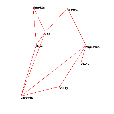
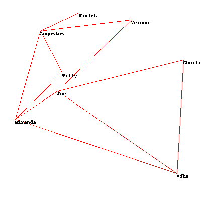
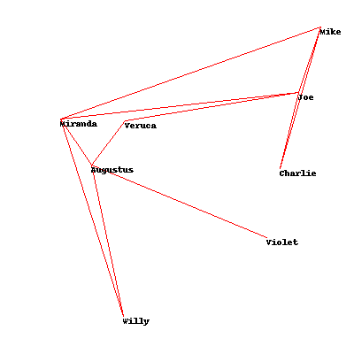
Social Network Graphs
The third and final problem concerns the problem of producing a readable graph. The graph is supposed to represent connections between users in a social network. In order to make the graph readable, we want to ensure that the connecting lines don't cross, as that would make even a simple graph hard to read.
The author acknowledges that the math for locating crossing lines is beyond the scope of the book, but he still supplies us with a usable cost function - cross_count. As in the other problems, we want to optimize the location of each node so that the minimum number of lines cross. Sounds familiar by now, doesn't it?
In [1]: import optimization
In [2]: import socialnetwork
In [3]: solution_random = optimization.random_optimize(socialnetwork.domain, socialnetwork.cross_count)
In [4]: socialnetwork.cross_count(solution_random)
Out[4]: 0
In [6]: solution_annealing = optimization.random_optimize(socialnetwork.domain, socialnetwork.cross_count)
In [7]: socialnetwork.cross_count(solution_annealing)
Out[7]: 0.2527383323092238
In [8]: solution_genetic = optimization.genetic_optimize(socialnetwork.domain, socialnetwork.cross_count)
In [9]: socialnetwork.cross_count(solution_genetic)
Out[9]: 0.2527383323092238
Comments
Add new comment