Programming Collective Intelligence chapter 7 notes

Published: 2014-04-29

Tagged: python readings guide

Chapter 7 of Programming Collective Intelligence (from here on referred to as The Book) is about decision trees. Decision trees, in the machine learning sense, are a great way to trace decisions and, more importantly, their causes. Furthermore, after training a decision tree, it is possible to use it to classify new observations. All the code needed for this note can be found here.

The Theory

The example provided by The Book is data about user interactions on a website and the results of those interactions - purchasing a Basic or Premium plan or not purchasing anything at all. The data that is provided covers the referrer, the location, whether they read the faq, and finally how many pages they checked out on the imaginary example website. The last column is the user's action, which I outlined just above.

The easiest way to illustrate what kind of information a decision tree would supply us is to present the tree itself:

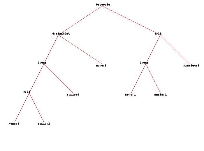
This is an image generated by treepredict.py and is based on the small dataset. Looking at the top we see the root node that is labled "0:google". This means that the most important factor determining which of the three outcomes users chose was the fact that they came from a google search or not. The "0" simply tells us the column. Here's an important part to keep in mind - this kind of tree only grows two branches: false on the left and true on the right. This means that going one level lower, the node on the right ("3:21") is what happens when a user arrives at the site from google. The node on the left tells us what happens when the user doesn't arrive from google.

For those that didn't arrive from google, the next most important factor is whether they came from slashdot. If true, the branch leads to "None", which is a result or class. So traffic coming from slashdot is unlikely to purchase any plan. Keeping to the left-most part of the tree, we see that if the traffic didn't come from slashdot and read the faq ("2:yes"), then it was likely they purchased a basic plan. Going further - those that didn't read the faq (going one level down, using the false branch) finally branch into those who viewed more than 21 pages on our site and those that didn't. Those that did - sometimes purchase the basic plan. Those that don't - don't purchase anything.

Going back up to the second level right branch ("0:google" -> "3:21"), we notice that those users that viewed more than 21 pages purchased the premium plan. Those that didn't, but read the faq then purchased a basic plan. Those that didn't view enough pages and didn't read the faq don't purchase anything.

We can also follow the tree from the bottom to the top. Doing this it's easy to see that users who buy the premium plan came from google and viewed quite a few pages before buying the premium plan. Those that didn't view enough pages, but read the faq went for the basic plan. Those that came from slashdot didn't purchase anything. This imaginary company should then focus on acquiring traffic from google and by providing a good many pages of quality content to hook the most valuable users. Additionally, it looks like the faq is a worthwhile investment. Notice that the location of the traffic didn't play any role. Interesting.

Quite a lot of insight, right? It's a wonder we don't see more of these. Let's get down to how it actually works.

The Fun

Some More Theory

The way to represent a decision tree (according to The Book) in the code is similar to how it looks on that image above - an actual tree. Trees in computer science, at least according to my experience, mean nodes and recursion. Before I delve into the code side of things, let's see why decision trees work. This will hopefully make it easier to explain the code itself.

The abstract idea at the lowest level of this construct is entropy. The flip side to this idea is information gain. An increase in information gain is a decrease in entropy. An increase in entropy is a decrease in information gain. In our case, we'll stick to calculating the entropy of data and our goal will be to minimize it. Doing so increases information gain.

As we saw in the image above, each level of the decision tree branches into true and false branches. These branches test a condition and branch out in one of those ways. In the case of strings, our code will branch on the condition of str1 == str2. This will lead to dividing our dataset into rows that hold str2 and those do not. In the case of numbers (integers and floats), our code will branch on the condition of val1 >= val2. As in the case of strings, this will divide our set into rows that are equal to or greater than val2 and those that are not.

Now, we will combine the previous two concepts into one: our code will iterate the data column by column and each time it will divide the data into two different sets many times. It will then calculate the entropy for each resulting pair of sets. When the entropy is the lowest for a given column, the value by which the column was divided is used to branch the tree. This is because this value provides the most information gain (lowest entropy). In our case, the entropy is calculated using the results column - after obtaining a pair of sets, we check the entropy of their related results. As the root node shows, it seems that dividing our dataset into the sets 'google' and 'not google' produces the lowest entropy score for this pair of sets. We then repeat this process for the newly created nodes until we reach the end of our dataset.

An important part of decision trees is pruning. The algorithm for building the decision tree will continue on splitting datasets even if the split doesn't lead to information gain. We can get rid of these useless notes by pruning the tree. The prune function is fairly simple - it checks if the difference in entropy between both branches and the sum of both branches divided by two is larger than a user supplied max_gain value - if it isn't than the nodes are unlinked from the tree.

The Meat

As I mentioned before, according to my experience, the best way to represent a tree structure is with an actual tree of nodes. If you already know about trees then you can safely skip this section. If you're totally new to this concept, I recommend this chapter of a free book on python algorithms and data structures to get a better idea what a tree is and to read on!

The basis of our decision tree will be the DecisionNode class. Objects of this class will hold data about what column the node describes, which value was the column divided by (value), the true and false branches if there are any, and the results if there aren't any branches.

The magic happens in the build_tree function, which as the name suggests, digests input data and spits out a decision tree made up of DecisionNode objects. I annotated the code as much I could. This function follows the plan laid out in the last paragraph of the previous section - iterate through columns and rows, find the value which splits the data in a way providing the most information gain, create the branches, repeat.

Getting Results

The treepredict.py module comes with many helpful utility functions that help with exploring our decision tree. I'll start off with the coolest one first:

classify and md_classify - these two functions both take a new observation and a tree and classify the observation according to the tree. The difference between these two function is that the second one handles missing data:

In [1]: import treepredict
In [2]: tree = treepredict.build_tree(treepredict.my_data)
In [4]: treepredict.classify(['google', 'USA', 'no', 23], tree)
Out[4]: {'Premium': 3}
In [5]: treepredict.classify(['google', 'USA', 'no', 10], tree)
Out[5]: {'None': 1}
In [6]: treepredict.classify(['google', 'USA', 'yes', 10], tree)
Out[6]: {'Basic': 1}
# Missing data - location
In [7]: treepredict.md_classify([None, 'France', 'yes', 25], tree)
Out[7]: 
{'Basic': 1.2422360248447204,
 'None': 0.6987577639751552,
 'Premium': 1.3695652173913044}
In [8]: treepredict.md_classify([None, 'France', 'yes', 10], tree)
Out[8]: {'Basic': 1.7857142857142856, 'None': 1.0044642857142856}
In [9]: treepredict.md_classify([None, 'France', 'no', 10], tree)
Out[9]: {'None': 0.8999999999999999}
# Missing data - other
In [10]: treepredict.md_classify([None, 'France', None, 10], tree)                                            
Out[10]: {'Basic': 0.8198495412121967, 'None': 0.4611653669318606}
In [11]: treepredict.md_classify(['google', 'France', None, None], tree)
Out[11]: {'Basic': 0.125, 'None': 0.125, 'Premium': 2.25}

prune - as I mentioned before in the theory section of this post, pruning is needed to rid our tree of nodes that do not contribute to information gain. This function doesn't really do much for our tiny example dataset, but it's definitely something to keep in mind when working on real world problems.

draw_tree - this function uses the PIL and the draw_node function to create a jpg file with a graphical representation of our tree. The output is actually what I used as the tree image in the beginning of this post. Using it is as simple as:

In [12]: treepredict.draw_tree(tree, jpeg='d_tree.jpg')

print_tree - this function prints out a simple ascii representation of a tree. Potentially useful for quickly diagnosing parts of a tree, but I think it would be rather unwieldy in a real world scenario for big trees:

In [13]: treepredict.print_tree(tree)
0:google? 
T-> 3:21? 
    T-> {'Premium': 3}
    F-> 2:yes? 
        T-> {'Basic': 1}
        F-> {'None': 1}
F-> 0:slashdot? 
    T-> {'None': 3}
    F-> 2:yes? 
        T-> {'Basic': 4}
        F-> 3:21? 
            T-> {'Basic': 1}
            F-> {'None': 3}

get_width and get_depth - these are used by the draw_tree function and are run of the mill functions to obtain the dimensions of a tree, but I thought it would be cool to mention these. I really enjoyed this recursive solution to the problem of finding out the size of a tree and it's great for someone who wants to brush on their recursion/data structures knowledge.

In [14]: treepredict.get_width(tree)
Out[14]: 7
In [15]: treepredict.get_depth(tree)
Out[15]: 4

Afterword

Decision trees were hella fun. This reminds me of naive Bayes' in that both of these ways of working with data are easy and quite intuitive. They may not be as flexible as neural networks or as powerful as support vector machines, but they are possible to implement, out of memory (with a few tweaks) in an afternoon. This makes them even easier to understand since they're no longer a magical black box for dumping data in and getting data out.

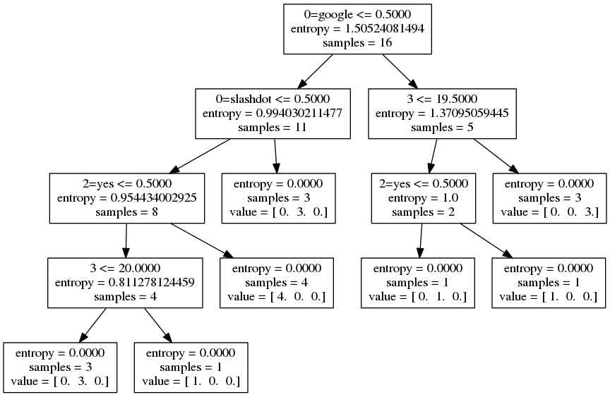
P.S I added a simple scikit-learn example that accomplishes the same classification task except in a mere < 20 lines. Note that scikit-learn decision trees have no built-in way of pruning themselves. This is what the output looks like: