Programming Collective Intelligence chapter 8 notes

Published: 2014-05-11

Tagged: python readings guide

Chapter 8 of Programming Collective Intelligence(from here on now referred to as The Book) takes us into the fun world of k-nearest neighbors. As usual, I annotated the code to make the principles easier to grasp. To perform some of the code examples for this chapter, you might need to copy over optimization.py from chapter 5 and comment out the code responsible for reading in any files. This is due to some interactive exercises requiring to optimize a cost function using annealing or genetic optimization.

What it is and How it Works

The k-nearest neighbors algorithm can be used for both classification and regression. The Book focuses on the latter part using a randomly create set of data related to wine (rating, price, age, and more later). I'll use this example to illustrate the principles behind kNN.

Suppose you have a set of 300 wines. You know both the age, rating, and price of each wine. You want to use this data to evaluate the price of a wine having only the age and rating. How do you do this?

Somewhat similarly to Chapter 2, you figure out which wines from your set of known wines are the most similar to this mystery wine. You select a k number of similar wines to base your prediction on, hence the name k-nearest neighbors. Choosing the correct number of neighbors to evaluate depends on the data itself. If the number is too big, the nearest neighbors stop having anything to do with the mystery wine. If the number is too small, we're leaving out precious information that influences the prediction.

To increase the accuracy of our prediction, the chapter introduces weights. If the nearest neighbor is close, but the second neighbor is far away, we'll make the first neighbor have a strong influence on our prediction whereas the far away neighbor will have a weaker influence.

As you can see, this algorithm is very easy to implement and play around with. I have also included the same algorithm implemented using scikit-learn's KNeighborsRegressor, which shortens the code a lot and probably makes it perform faster too.

Testing!

This chapter introduces simple cross validation. Cross validation helps us to test how accurate our predictions so that we can tweak our algorithms to increase accuracy. In this simple case, we split our data set into a training set and a test set. The training set, as the name implies, is used to train our algorithm. The test set is then used to check how accurately the classifier or regressor performs. In this chapter, we split out 5% of the data set to form the test set. In other cases we might split up substantially more, say, 25% of the whole data set. For the curious, a slightly more elaborate testing scheme is to split the data into three sets: training, validation, and testing. In this case, the validation set is used to train different algorithms with different parameters to pick the best one.

How to explore the code

Let's explore the code interactively a bit. We'll start off with the first simple example where our wine only has a rating and age. Then we'll move onto the second set, where the wine also has a bottle capacity as well as an aisle. Last but not least, we'll work on a set where some wines have been discounted. We'll use kNN to discern this fact.

In [1]: import numpredict
In [2]: data1 = numpredict.wine_set_1()
In [3]: numpredict.knn_estimate(data1, (95.0, 3.0))
Out[3]: 19.202224959807165
In [4]: numpredict.knn_estimate(data1, (95.0, 5.0))
Out[4]: 35.982267167962014
In [5]: numpredict.wine_price(95.0, 3.0)
Out[5]: 21.111111111111114
In [6]: numpredict.wine_price(95.0, 5.0)
Out[6]: 31.666666666666664

First we check the price of a 3 year old wine rated at 95 points, then a 5 year old wine rated at 95 points using the default of k = 3. Then we cheat and use the price-generation function to obtain the real price of those two wines. As we see, the predictions weren't too far off. Try out setting k = 4 - the results will get slightly more accurate. In the real world, we won't have a way to cheat like this. This is where cross validation will come in a bit later. Let's check out the weighted_knn function for both of these hypothetical wines using different k:

In [11]: numpredict.weighted_knn(data1, (95.0, 3.0), k=3)
Out[11]: 19.27638129038519
In [12]: numpredict.weighted_knn(data1, (95.0, 3.0), k=5)
Out[12]: 17.656159794841898
In [13]: numpredict.weighted_knn(data1, (95.0, 3.0), k=2)
Out[13]: 24.240207543612822
In [14]: numpredict.weighted_knn(data1, (95.0, 5.0), k=2)
Out[14]: 31.223695643676766
In [15]: numpredict.weighted_knn(data1, (95.0, 5.0), k=3)
Out[15]: 35.98521381850595
In [16]: numpredict.weighted_knn(data1, (95.0, 5.0), k=5)
Out[16]: 34.44516826960828

Interesting. Using k = 3 gives a more accurate result for the younger wine whereas k = 2 gives a more accurate result for the older one. There's one more parameter we can tweak - the weighing function that's passed in to weighted_knn as weight_f. The default is the Gaussian function, but The Book supplies us with two other ones: inverse_weight and subtract_weight. It's worth to explore weighted kNN and this simple data set using those other functions as well.

Validation!

Now we'll finally check out cross validation. As I mentioned before, we first have to break the original set of data into a training and testing set. We'll use these sets to measure the sum of errors for various parameters such as the k number as well different algorithms (knn_estimate vs weighted_knn):

# Using knn_estimate with k = 3
In [18]: numpredict.cross_validate(numpredict.knn_estimate, data1)
Out[18]: 451.63664602373467
# Using a lambda function to wrap knn_estimate to use k = 5
In [19]: numpredict.cross_validate(lambda data, vec: numpredict.knn_estimate(data, vec, k=5), data1)
Out[19]: 464.34538086471855
# Using weighted_knn with k = 5
In [20]: numpredict.cross_validate(numpredict.weighted_knn, data1)
Out[20]: 539.5957793832488
# Using weighted_knn with k = 3
In [21]: numpredict.cross_validate(lambda data, vec: numpredict.weighted_knn(data, vec, k=3), data1)
Out[21]: 566.069846871194
# Using weighted_knn with k = 3 and inverse_weight as the weighing function
In [22]: numpredict.cross_validate(lambda data, vec: numpredict.weighted_knn(data, vec, k=3, weight_f=numpredict.inverse_weight), data1)
Out[22]: 453.0526769849885

Optimization!

Next up is a short detour into combining optimization (chapter 5 and kNN. We'll optimize the scaling of different features using the second wine set that includes bottle capacity and the aisle number. Looking at wine_set_2(), we see that bottle capacity plays a role in determining the price, but aisle doesn't - it's just a random number at this point. Noise. Knowing this, we'd expect the aisle variable to be scaled low or even down to zero. The cost function will use cross validation to determine the optimal set of weights - minimize the cost and thus minimize the errors.

In [2]: import optimization
In [3]: data2 = numpredict.wine_set_2()
In [4]: optimization.annealing_optimize(numpredict.weight_domain, cost_function, step=1)
Out[4]: [13.0, 18.0, 11, 7.0]

Let's try this out using the slower but potentially better genetic_optimize function (REALLY SLOW):

In [8]: optimization.genetic_optimize(numpredict.weight_domain, cost_function, step=2)
Out[8]: [16, 20, 2, 17]

This makes more sense. The rating, age, and capacity are pretty important whereas the aisle is much less important. Scaling is important to line up features of different sizes ie. age (0-10) and capacity (375-3000). This will ensure that the distances between neighbors are properly represented. What is more, as in the case of the aisle, scaling it to 0 will not not affect the distances since the aisle doesn't play any role in determining the price. This is extremely useful in getting rid of useless features. For the curious, scipy has a set of optimization functions: scipy.optmize.

Probability!

Finally, we get to the part about uncovering hidden features in a data set. This time we'll use wine_set_3() to obtain a set where a random number of wines are discounted and this data is not reflected in the features (rating, age). This opens up the fascinating world of probability distributions and how to apply them to kNN.

To start, we'll use prob_guess to check out the probability that a mystery wine falls into a range of prices, using the wine_set_1() data:

In [26]: numpredict.prob_guess(data1, [80, 5], 10, 50)
Out[26]: 0.40102767213592055
In [27]: numpredict.prob_guess(data1, [80, 5], 20, 50)
Out[27]: 0.2049517979053861
In [28]: numpredict.prob_guess(data1, [80, 5], 10, 30)
Out[28]: 0.19607587423053444
In [29]: numpredict.prob_guess(data1, [80, 5], 10, 40)
Out[29]: 0.19607587423053444

We'll use this function along with matplotlib to graph this data to make it more readable. First, we'll get a cumulative probability graph. This graph shows the range that a wine might cost:

In [33]: numpredict.cumulative_graph(data3, [95.0, 5.0], 120)

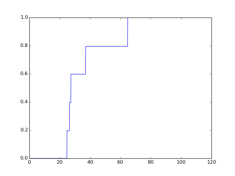
Reading this graph, we see that the probability that our mystery wine has 0% chance to cost less than 25$ and a 100% chance that it costs less than 65$. Looking at the steep rise on the left side of the graph, we see that there's a 60% probability that the wine costs less than 27$. Combining this information, we can guess with a 60% chance of success that this wine costs between 25$ and 27$. Insanely cool.

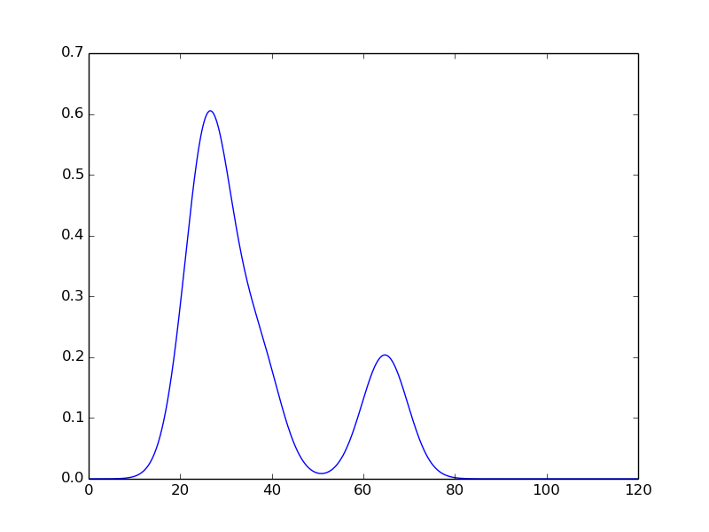
Going one step further, why not plot a nice smooth curve that ties in prices and their probabilities?

In [34]: numpredict.probability_graph(data3, [95.0, 10.0], 120)