Programming Collective Intelligence chapter 9 notes

Published: 2014-05-17

Tagged: python readings guide

Chapter 9 of Programming Collective Intelligence(from here on now referred to as The Book) introduces us to support vector machines. The annotated code can be found here. The Book doesn't go into many of the mathematical details underlying SVMs and instead gives us an intuitive introduction. The chapter builds a very simple classifier which illustrates the principles behind SVMs and then goes on to use LIBSVM. I decided to avoid the last step and instead opted to use scikit-learn's svm module to get the job done. For those that want to get a better grasp on SVM's, I recommend Andrew Ng's excellent Coursera Machine Learning course, which delves deeper into the math behind SVMs.

A Light Intro

In the most basic sense SVMs introduce a line to divide data and use that division to classify that data. What helps SVMs to go above simple logistic regression is that SVMs strive to maximize the margin between the classes of data. The image below illustrates a classification when the margin is not optimal:

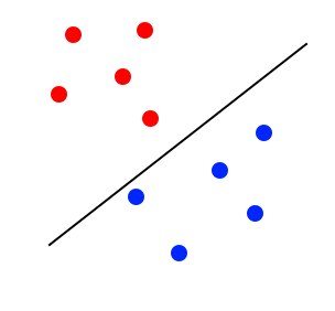
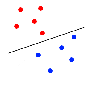
The margin looks to be too close to the blue classifier. It will lose accuracy because some blue points will be classified as red. The image below illustrates a better margin than the one before:

For this chapter, we'll be using two datasets. Both relate to making matches between people such as on a dating website. The first set (agesonly.gz) only holds age data and whether the two people made a successful match. The second set (matchmaker.gz) contains the age as well whether the person wants children, their interests, and geographical location. The first set will be used to perform a simple linear classification whereas the second will be food for a non-linear classifier as well a demonstration of feature scaling.

Exploring the Code

We'll start off with simple linear classification using the first set of data:

import advancedclassify
num = advancedclassify.load_match('agesonly.gz', all_num=True)
avgs = advancedclassify.linear_train(num)
advancedclassify.dp_classify([30, 30], avgs)
#[Out]# 1
advancedclassify.dp_classify([25, 30], avgs)
#[Out]# 0
advancedclassify.dp_classify([30, 25], avgs)
#[Out]# 1

According to our classifer, a man and a woman of the same age are ok, but a younger man and older woman (2nd classification) won't work. If you flip the ages and have an older man and a younger woman - it works.

For the second dataset we have to do a bit more work. First, the load_numerical function will transform the raw data into pure numerical data. It'll transform things like 'yes', 'no', 'cats:airplanes:mario' into numbers. The yes/no questions can easily be fit into a boolean 0 or 1, whereas the interests are simply summed up - if two people share two of the same interests than they'll have a "2" in the appropriate column. The data set also contains each person's location, which can be turned into the distance and thus provide more information for our classifier. However, this requires translating a physical address into a set of coordinates and then measuring the distance, for which I couldn't find a decent offline solution and I didn't want to use an online API for this, so I made it a random 0 or a 1.

After taking care to transform the data into something usable, we also have to scale the data. This is a necessary step because the classifier works by calculating the distance between data points and vastly different feature would have a bad affect on the final accuracy. An easy way to understand this is to visualize two features on a Cartesian plane where the x-axis is feature 1 and the y-axis is feature 2. If both features are scaled to the range of between 1 and 10, the rate of change of the distance between these features will be similar to each other ie. a change of 2 units in feature 2 will have he same affect on the distance as a change of 2 units in feature 1. Imagine how this would work if features weren't scaled - say feature 1's axis would be a range between 1 and 10 whereas feature 2's axis would be between 1 and 10000. A change of 2 units in feature 1 would mean a large change in distance compared to a change of 2 units in feature 2.

Alright, let's give the code a whirl:

import advancedclassify
num = advancedclassify.load_numerical()
scaled, scale_f = advancedclassify.scale_data(num)
avgs = advancedclassify.linear_train(scaled)
ssoffset = advancedclassify.get_offset(scaled)
advancedclassify.nl_classify(scale_f(num[0].data), scaled, ssoffset)
#[Out]# 0
num[0].match
#[Out]# 0
advancedclassify.nl_classify(scale_f(num[1].data), scaled, ssoffset)
#[Out]# 1
num[1].match
#[Out]# 1
advancedclassify.nl_classify(scale_f(num[2].data), scaled, ssoffset)
#[Out]# 0
num[2].match
#[Out]# 0
# Compare two similar people where the man doesn't want children:
advancedclassify.nl_classify(scale_f([28.0, -1, -1, 26.0, -1, 1, 2, 0.8]), scaled, ssoffset)
#[Out]# 0
# Compare two similar people where both of them want children:
advancedclassify.nl_classify(scale_f([28.0, -1, 1, 26.0, -1, 1, 2, 0.8]), scaled, ssoffset)
#[Out]# 1

Scikit-learn

At this point, The Book goes onto introduce the excellent LIBSVM library, which I chose to avoid using for the simple reason that I had scikit-learn's SVM functionality already set up and at my fingertips. The code is only a handful of lines long, so it's really easy to play around with different datasets and see what results you get. You can check out this code here.

I run the second data set (matchmaker.gz) through scikit-learn's SVM implementation at the default settings. I then run the same prediction on a pair of similar people where in the first case the man doesn't want children and in the second case where both of them want children. I also use the score function on a small test part of the general dataset to rate it's accuracy and usually get between 70 and 80 percent. That's ok-ish and I assume I could improve the accuracy by either using a real measure of distance or discarding distance altogether. I could also improve the way the interests are transformed into numerical features.

SVM's are definitely a much more mathematical and complex topic and they're not as easy to implement as some previous algorithms (naive Bayes' or k-nearest neighbors). But they perform much better in cases where features have more complicated relationships or if there's quite a large number of features.